
Introduction#
Because MapReduce was slow for machine learning, researchers at UC Berkeley started Spark.
Here is one SQL query on New York City taxi trip data, stored in an Iceberg table.
SELECT EXTRACT(MONTH FROM tpep_pickup_datetime) AS month,
       count(*) AS trips,
       avg(fare_amount) AS average_fare
FROM trips
WHERE tpep_pickup_datetime >= TIMESTAMP '2024-01-01 00:00:00'
  AND tpep_pickup_datetime < TIMESTAMP '2025-01-01 00:00:00'
GROUP BY 1
ORDER BY 1
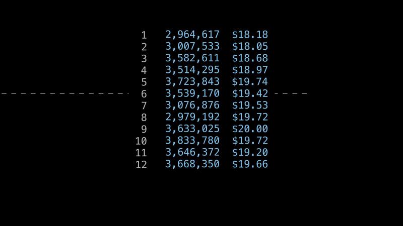
It counts New York’s taxi trips in each month of 2024 and averages their fares. The table holds 41 million trips in 712 MB of Parquet files. On average, each month has about 3.4 million trips. The query needs only two of the table’s 19 columns. On disk, they take 233 MB. Because the pickup time has about 20 million different values, it compresses poorly. It alone takes 187 MB.
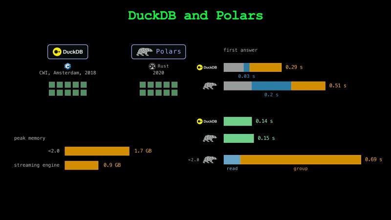
We run the query with DuckDB, Polars, and Spark on a MacBook with 10 cores. DuckDB answers in 0.29 s. Polars answers in 0.51 s. Spark answers in 5.66 s.
On one laptop, Spark is the slowest of the three. Then why do teams run Spark?
Engines and Tables#
Managing big data takes three jobs: storing the data, keeping its metadata, and processing it. Parquet files store the data. Iceberg keeps the metadata. The programs that do the processing are called engines. DuckDB, Polars, and Spark are three of them.
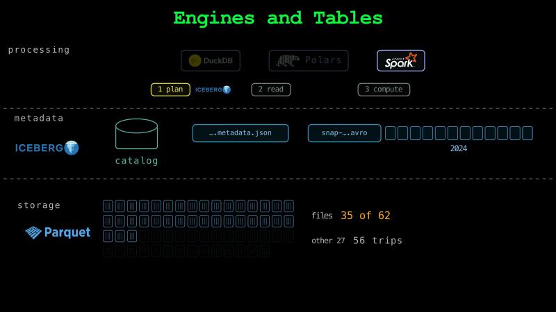
Every engine runs a query in the same three steps. First, the engine reads the catalog and Iceberg’s metadata files to plan which data files to read. We ask only for the trips of 2024. The engine uses Iceberg’s metadata alone to choose 35 of the table’s 62 data files. The other 27 files hold only the 56 trips from other years.
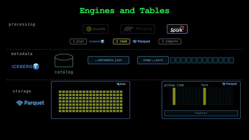
Second, the engine reads only the columns the query needs: the pickup time and the fare. Because a Parquet file stores each column in its own part of the file, the engine can skip the other 17 columns. The footer at the end of each file lists where each part starts. With Iceberg’s metadata, the engine can only skip whole files. An Iceberg table can also keep its data in Avro files. Because Avro stores data row by row, an engine that reads an Avro file reads every column.
Third, the engine computes the result by itself. It keeps the trips of 2024, groups them by month, counts them, and averages each month’s fares.
Because DuckDB, Polars, and Spark follow the same Iceberg specification, they read the same metadata and the same Parquet files.
To Distribute or Not#
The three engines differ in how they compute. DuckDB and Polars run inside our Python process. They split the rows into small groups, which are called batches. Each of the laptop’s 10 cores takes the next batch. For our query, each core keeps the trips of 2024. It counts the trips by month and adds up each month’s fares. When no batches are left, the engine adds up the counts and sums of the 10 cores.
The processing stays within one process on one machine.
Spark runs in its own Java process. It can split the work across many machines. Spark splits the data files into parts. For each part, it counts the trips and adds up each month’s fares. Before Spark adds up a month’s counts and sums, it may have to send them over the network to one machine.
DuckDB and Polars#
DuckDB started in 2018 at a research institute in Amsterdam. Its makers built a SQL database for analysis. Like SQLite, DuckDB runs inside the program that uses it. Polars started in 2020 as a DataFrame library built to use every core of one machine, an alternative to pandas. DuckDB is written in C++. Polars is written in Rust. Both use all 10 cores of the laptop. Why is DuckDB faster than Polars on our query?
First, Polars opens Iceberg tables with a Python library called PyIceberg. DuckDB opens them with its own C++ code. In each run, loading PyIceberg and opening our table took 0.2 s. Loading DuckDB’s Iceberg reader and opening the table took 0.03 s.
Second, DuckDB’s engine is only a little faster. When we run the query 10 more times without restarting the engines, DuckDB’s median is 0.14 s. Polars’ median is 0.15 s. Since version 2.0, Polars runs queries in batches with its default engine, which is called the streaming engine. Because the streaming engine holds only a few batches in memory at a time, it can also run a query on more data than the machine’s memory holds. Polars’ older engine first reads all 41 million trips into memory. Then it groups them. With that engine, our query took 0.69 s. At its peak, the process used 1.7 GB of memory. With the streaming engine, its peak was 0.9 GB.
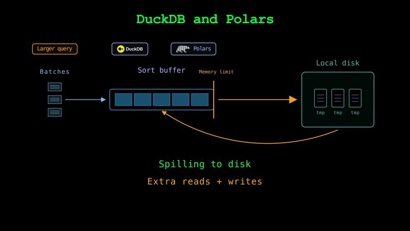
For larger queries, operations such as sorting may need to keep more data than fits in memory. DuckDB and Polars can write some of that data to temporary files and read it back later. This is called spilling to disk. The extra reads and writes take time.
Google File System and MapReduce#
Some data is too big for one machine. It has to be stored and processed on many machines. In 2003, Google described a file system called the Google File System. It splits each file into blocks of 64 MB. It keeps three copies of each block on different machines. When a machine fails, its blocks still have two copies on other machines. One main machine keeps the list of each file’s blocks and where they are.
In 2004, Google described a way to process those files on the machines that store them, which is called MapReduce.
A MapReduce job runs in two steps, which are, unsurprisingly, called map and reduce. In the map step, MapReduce tries to process each block on a machine that stores it. Most of the input doesn’t travel over the network. The map step gives every record a value to group it by, which is called a key. For our query, the key is the month. In the reduce step, the records with the same key go to one machine. The machine that gets January’s records adds up January’s fares.
Hadoop#
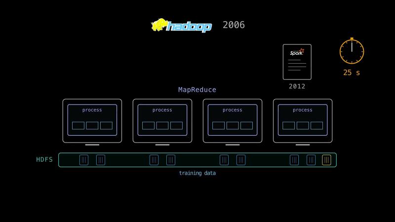
In 2006, a project called Hadoop rebuilt both of Google’s systems as open source. Hadoop’s file system is called HDFS. Hadoop MapReduce runs its jobs on the same machines. Why was MapReduce slow for machine learning?
Many machine learning algorithms read the same training data many times. One read of all the training data is called an epoch. With Hadoop, each epoch is a separate MapReduce job. Each job runs its work in new processes on the machines. The processes end before the next job starts. So, a job can pass data to the next job only through files. The files are usually in HDFS. Every job reads all the training data again from the files. Starting the new processes also takes time. In a Spark paper from 2012, a Hadoop job that did no work took 25 s.
How Spark Works#
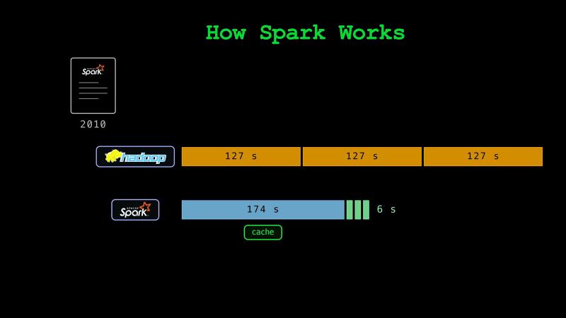
In order to address these limitations, Spark was created. Spark became open source in 2010 and moved to the Apache Software Foundation in 2013. Spark’s worker processes keep running from the start of a program to its end. So, a program can ask each worker to keep its part of the data in memory. Spark’s copy of the data in memory is called a cache. In the next epoch, Spark tries to send the work on each part to the worker that holds that part. While the cache stays in memory, the program doesn’t read the files again in later epochs.
In Spark’s first paper from 2010, a machine learning program on Hadoop took 127 s an epoch. On Spark, the program filled the cache during the first epoch. The first epoch took 174 s, but every later epoch took 6 s.
Cache and Lineage#
Let’s do a local test that trains for 10 epochs on 39.7 million trips to learn how the fare grows with the distance. When our program reads the files in every epoch, the median epoch takes 0.47 s. Filling the cache takes 0.88 s. Then the median epoch takes 0.18 s.
Spark’s cache holds the trips after they are decoded and filtered. When a worker machine fails, the data in its memory is lost. For each part of its data, Spark keeps the steps that made the part, which are called its lineage. After a failure, Spark runs those steps again and rebuilds only the lost parts.
How Spark Runs a Query#
A Spark program runs one main process and many worker processes. The main process is called the driver. The worker processes are called executors. The executors can run on other machines.
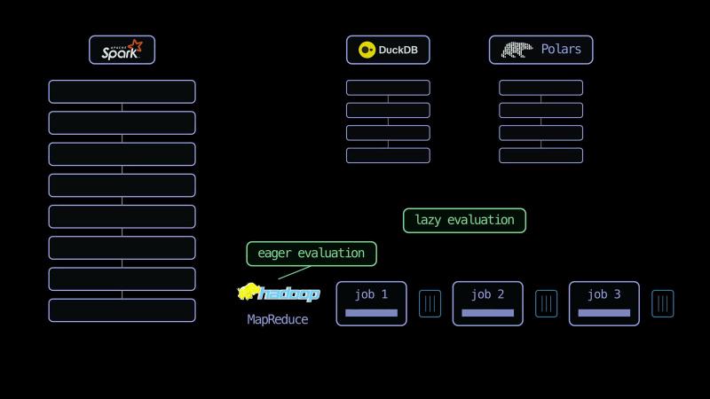
When we give Spark our query, it builds a plan without reading any trips. Running a plan only when its result is asked for is called lazy evaluation. You can chain lazy operations together, which will then be optimized further by the engine. DuckDB and Polars can also use lazy evaluation. Yet, Hadoop’s MapReduce runs each job as soon as the program submits it.
Query Plan#
Spark’s plan for our query has eight steps. We read them from the bottom up. The scan reads the pickup time and the fare from the 35 data files. A reader can also skip a Parquet row group whose pickup times all fall outside 2024. But every row group in our 35 files holds trips of 2024. Spark’s filter checks each of the 41 million trips and keeps the trips of 2024. Taking the month out of each pickup time is called a projection. A step that combines many rows into one result is called an aggregate. The first aggregate counts the trips and adds up the fares of each month in each part of the data. Sending each month’s counts and sums to one place is called an exchange. The second aggregate adds them up and divides the sum of the fares by the number of trips. The second exchange splits the months into ranges. The sort puts each range in order. Our 12 months fit in one range.
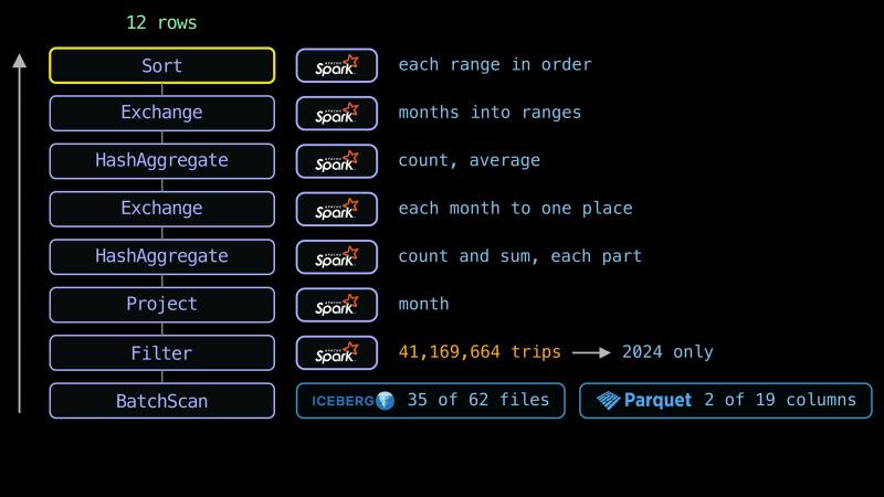
Of the eight steps, only the scan uses Iceberg or Parquet. It uses Iceberg’s metadata to choose the 35 files and Parquet’s layout to read only two columns. Spark runs the other seven steps by itself.
Tasks and Executors#
The driver splits the plan into small pieces of work, which are called tasks. The work is split into parts of about 16 MB. Our query starts with 47 tasks. Each task runs the first four steps of the plan on one part.
An executor runs one task at a time on each of its cores. On this laptop, the driver and one executor share one process. The executor uses all 10 cores. Once Spark is running, our query takes 2 s with one core and 0.48 s with 10 cores.
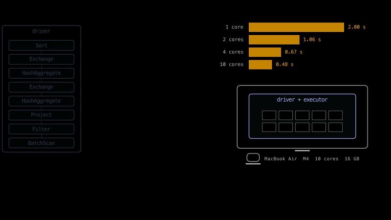
An executor is one process. A process uses the cores of one machine. Each machine that runs Spark’s tasks needs at least one executor. Java doesn’t always run well with more than 200 GB of memory. For a machine with more memory than that, Spark’s documentation suggests several executors.
Stages and Shuffles#
Moving the rows with the same key to the same task is called a shuffle. Each exchange in the plan is a shuffle. Hadoop’s MapReduce already used this name for the step between map and reduce. A shuffle can send rows between machines over the network.
During a shuffle, Spark can also spill a task’s working data to local disk when it doesn’t fit in memory.
The tasks that run with no shuffle between them are called a stage. Each shuffle ends one stage and starts the next.
Because every task added up its own rows first, our first shuffle moves only 64 rows of sums. Without these sums, the shuffle would move every one of the 41 million trips.
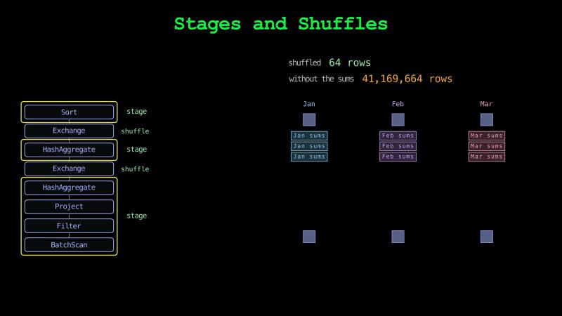
After the first stage, one task runs the second aggregate and samples the months to choose the ranges for the sort. Another task runs the aggregate again and sends the 12 months to the sort. The last task sorts them. In all, our query runs 50 tasks.
When One Machine Is Enough#
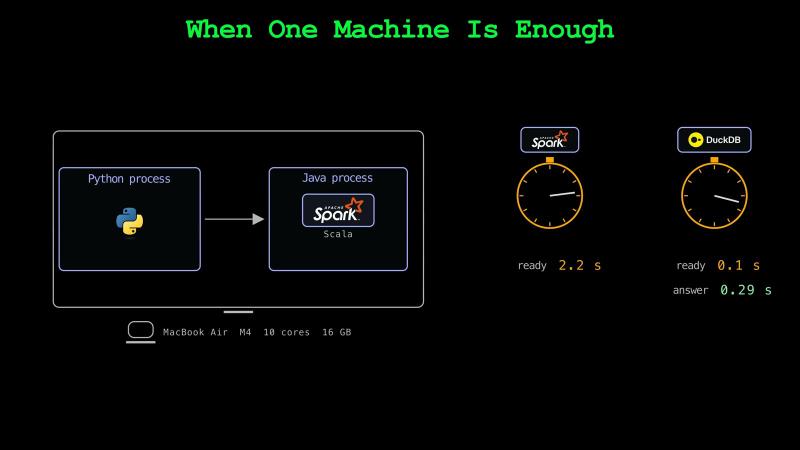
Spark is written in Scala. Scala programs run on the Java virtual machine. On this laptop, our Python program starts a Java process for Spark. In the test, Spark needed 2.2 s to start before it could read any trips. DuckDB was ready in 0.1 s and had its first answer at 0.29 s. Because Spark is built for many machines, it also plans stages, sends every task to an executor, and writes the shuffled rows to files between stages.
In 2023, a founding engineer of Google BigQuery described a study of queries from BigQuery customers who spent over $1,000 a year. The study found that 90% of the queries processed less than 100 MB of data.
Spark is worth its costs when the data is too big for one machine, or when one machine would take too long to process it. Then Spark runs the plan’s tasks on many machines and can rebuild the parts that a failed executor held.
Up Next#
We’ve seen how to work with data in a table and when to use single-machine solutions or distributed systems.
So far, we’ve assumed the data was already there. In the next part, we’ll explore how data gets into the table in the first place.
See you there!
Taxi trip data from the NYC Taxi & Limousine Commission. Rust logo from the Rust Foundation, CC BY 4.0.