Big-O Basics for Time and Space Complexity

Table of Contents

DSA Despite AI - This article is part of a series.

Part 1: This Article

Part 2: Arrays vs ArrayLists vs Linked Lists (Does Python Even Have Arrays?)

Introduction
#

This function removes duplicates from a list.

def dedupe(items: list[int]) -> list[int]:
    out: list[int] = []
    for x in items:
        if x not in out:
            out.append(x)
    return out

On a list of a thousand different items, it takes 2.5 ms. On a hundred thousand, it takes 27 seconds. That’s a hundred times the data, but more than ten thousand times the duration.

There’s one loop in this code. So where is the time spent?

An AI assistant can write a slow or a fast version of this function, and we should be able to do the same.

Counting Steps
#

To see where the time goes, we count steps instead of seconds. Seconds depend on the hardware. Steps depend only on the code and its input.

For n items, the loop runs n times. Inside it, the membership check looks like a single step, but it’s a loop of its own. Python compares x with each item in the output list it’s building, one by one, until it finds a match or reaches the end.

When every item is new, the output list grows by one each time, so the checks take zero comparisons, then one, then two, up to n − 1.

That’s about n²/2 in total, which is typical of two nested loops. In our example, a thousand items need half a million comparisons, and a hundred thousand need five billion.

Big-O Notation
#

The exact count matters less than how it grows with n, and that’s what Big-O notation describes.

Big-O keeps the fastest-growing term and drops constant factors, so n²/2 becomes O(n²).

The common growth rates have names. Constant time stays the same for any n. Logarithmic time grows by one step each time n doubles, because log n counts how many times n can be halved. Linear time grows in proportion to n. Linearithmic time is n times log n, which grows faster than both linear and logarithmic time. Quadratic and cubic time grow with the square and the cube of n. Both are special cases of polynomial time. Exponential time doubles with every item added. Factorial time, n factorial, multiplies by n instead. As n grows, exponential and factorial pass all the others.

Our function is quadratic, so doubling n quadruples the work. If 20,000 items take one second, then 40,000 take four. This is why, in our dedupe example, a hundred times the data means a hundred squared, or ten thousand times the work.

Lists vs Sets
#

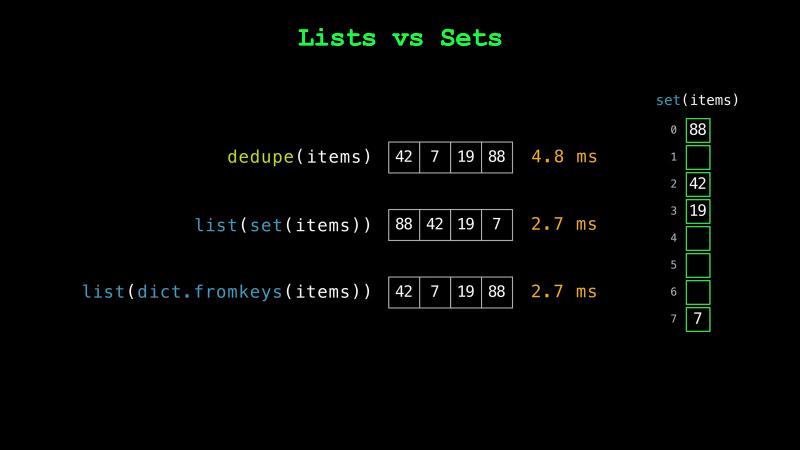
To make the function fast, the membership check has to stop scanning. A set can do that check without looking at every item.

It first turns each item into a number, called its hash. The hash points to the slot where the item belongs. For 53, the hash Python uses is the number itself. The slot is the remainder when the hash is divided by the number of slots. With eight slots, 53 modulo 8 gives slot 5.

So a membership check with a set looks in one slot instead of the whole list. Sometimes that slot holds a different item, which is called a collision, and the set tries another. The set keeps enough slots empty that a check takes only a few tries, so it’s O(1) on average.

def dedupe(items: list[int]) -> list[int]:
    seen: set[int] = set()
    out: list[int] = []
    for x in items:
        if x not in seen:
            seen.add(x)
            out.append(x)
    return out

With a set doing the check, a hundred thousand items take under 5 ms.

The in operator is still the same. But it asks a list to scan and a set to jump. The cost comes from the data structure, not the syntax.

Python can also remove duplicates in one line. Converting the items to a set and back to a list returns them in slot order, not in their original order. A dictionary’s keys are also unique, and they stay in the order they were added, so dict.fromkeys keeps the original order. Both still loop over every item, but in C instead of Python. At a hundred thousand items, they take under 3 ms, against under 5 ms for our loop.

dedupe(items) keeps the order 42, 7, 19, 88 at 4.8 ms, and list(dict.fromkeys(items)) keeps the same order at 2.7 ms, while list(set(items)) gives 88, 42, 19, 7, the order of the slots of set(items), at 2.7 ms

Complexity of Each Operation
#

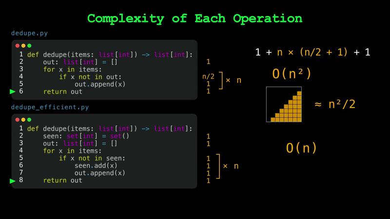
So far, we’ve counted the steps of one line. For the whole function, every line gets a price in steps. Let’s go line by line, starting with the slow version.

Creating the empty list takes the same time for any n, so it’s one step. The loop repeats the two lines inside it n times. When every item is new, the check scans an output list that grows from empty to n items, so it costs about n/2 comparisons. The append costs one step.

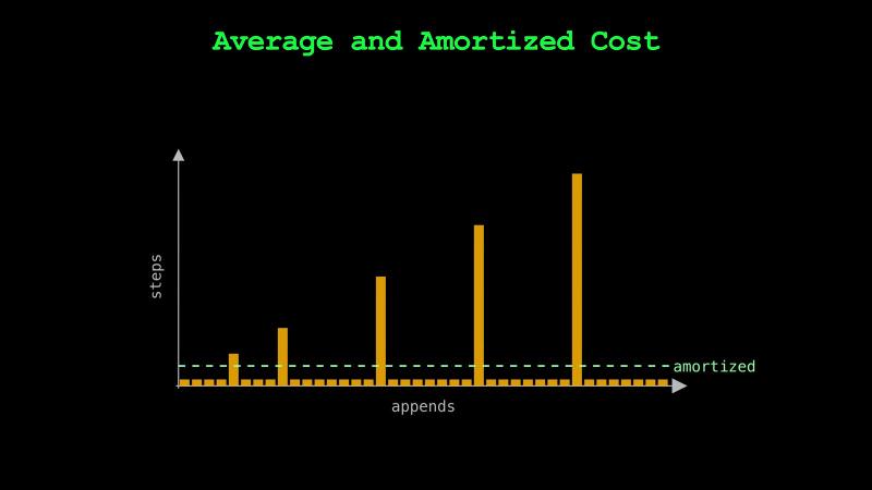
The append is one step because a list keeps spare room at its end, so it usually fills the next free cell. When the room runs out, the list moves into a bigger block in memory, with spare room in proportion to its size. A bigger list makes bigger moves, but fewer of them, so on average an append is still one step.

Finally, returning the list is one step too, since return gives back a reference to the list, not a copy.

The loop multiplies what’s inside it by n, and everything adds up to n²/2 + n + 2. The n²/2 is the count from before, and the other lines add n + 2. Big-O keeps n², so the slow version is O(n²).

In the fast version, the check, adding to the set, and the append are each one step on average. That’s 3n + 3, which is O(n).

dedupe.py costs 1, then n/2 and 1 inside the loop × n, then 1, which sums to 1 + n × (n/2 + 1) + 1 and is O(n²), beside the ≈ n²/2 staircase. dedupe_efficient.py costs 1 per line, with three of its lines × n, which is O(n)

Space Complexity
#

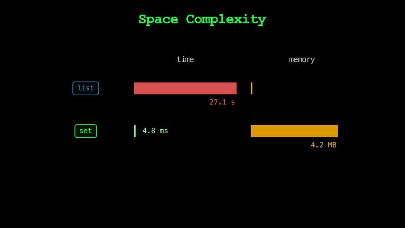
Time isn’t the only cost. The fast version also keeps a second collection, the set of items it has seen, which grows with every new item.

Memory is counted the same way, as a function of n, and that’s called space complexity. We usually count only the extra memory, beyond the input and the answer. Here the input is the list of items and the answer is the output list, so neither counts.

The slow version needs nothing else that grows with n, so its space complexity is O(1). The set of seen items grows with n, so the fast version’s space complexity is O(n). At a hundred thousand items, that set takes about 4 MB.

So the fast version trades memory for time, 4 MB for 27 seconds. Many speedups make this trade.

The list version’s time bar runs to 27.1 s while its memory bar is a sliver, and the set version’s time is a sliver at 4.8 ms while its memory bar runs to 4.2 MB

Bounds and Cases
#

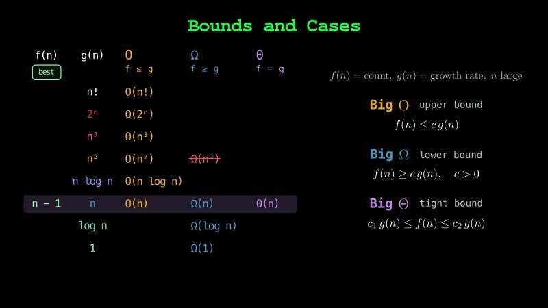
The slow version’s count of n²/2 assumed that every item is new. If every item is the same, each check finds its match at the first comparison, so there are only about n comparisons in total. The all-same list is the slow version’s best case, the input with the fewest steps. A list of all different items is its worst case, the input with the most.

Each case’s count can be bounded in three ways. Big-O is an upper bound, like less than or equal: the algorithm can’t take more than that much work. Big Omega is a lower bound, like greater than or equal: in the case we’re analyzing, it really does take at least that much work. Big Theta is both, like equals: the work grows like the rate, up to a constant factor.

A constant factor doesn’t change the rate, so 3n and 100n are both linear. Precisely, Big-O means the count stays below a constant times the rate once n is large. Big Omega means it stays above a positive constant times the rate, and Big Theta means both.

The worst case, n²/2, stays between a quarter of n² and n², so it’s Θ(n²). Every faster rate is an upper bound too, so it’s also O(n³), and every slower rate is a lower bound, so it’s also Ω(n). Only n² is both.

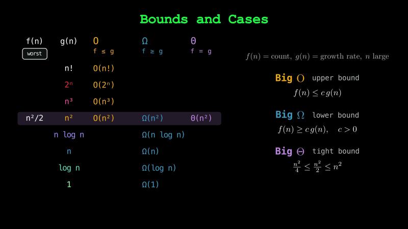
The worst case, f(n) = n²/2, on the n² row of a table of growth rates from n! down to 1: it is O(n²) up to O(n!), Ω(n²) down to Ω(1), and only Θ(n²). Beside the table, Big O is the upper bound f(n) ≤ c g(n), Big Ω the lower bound f(n) ≥ c g(n) with c > 0, and Big Θ the tight bound n²/4 ≤ n²/2 ≤ n²

The best case, about n comparisons, is Θ(n). It’s still O(n²), because n² grows faster, but it isn’t Ω(n²).

The best case, f(n) = n − 1, on the n row: it is now O(n) up to O(n!), Ω(n) down to Ω(1), and only Θ(n), while Ω(n²) is struck through in red

Average and Amortized Cost
#

A complexity given without a case usually means an upper bound on the worst case, which is why the slow version is O(n²). A set check’s O(1) describes its average case, the expected count over typical inputs.

The append’s one step is a different kind of average. An append sometimes copies the whole list, but over a long run of appends, the copies average out to a fixed cost per append. That’s called an amortized cost. It averages over the appends in one run, not over different inputs, so it holds for any input.

Steps per append: most bars are short, five copies stand taller and further apart each time, and a dashed line labeled amortized runs just above the short bars

Coding Interviews
#

Coding interviews ask for the time and space complexity of a solution. We can read both directly from the code. The same goes for code an AI assistant writes.

Big-O also tells us whether an idea is fast enough before we write it. Coding problems state their input size, like n up to a hundred thousand.

For example, at n = 100,000, a quadratic solution takes billions of steps. On the other hand, a hundred thousand can be halved about 17 times, so n log n is under two million. Python runs about 20 million simple steps per second, so that’s under a tenth of a second. Even with a constant factor of ten, it stays under a second.

So an input of a hundred thousand rules out quadratic solutions.

Both versions of this function pass a small test, but only one survives a large one.

In the next chapter, we’ll look at the most fundamental data structure, the array, and find out whether a Python list is one.

See you there!

DSA Despite AI - This article is part of a series.

Part 1: This Article

Part 2: Arrays vs ArrayLists vs Linked Lists (Does Python Even Have Arrays?)

Introduction#

Counting Steps#

Big-O Notation#

Lists vs Sets#

Complexity of Each Operation#

Space Complexity#

Bounds and Cases#

Average and Amortized Cost#

Coding Interviews#