How Python Works Under the Hood: Control Flow and Bytecode

Introduction

#

When we write a program, we are giving a computer instructions to perform some task. These instructions, such as if statements and loops, control the flow of the program. They let us make decisions and repeat actions.

 1
 2
 3
 4
 5
 6
 7
 8
 9
10
11
12

for n in [4, 8, 15, 16, 23, 42]:
    if n == 42:
        print(
            "Answer to the Ultimate Question of Life, "
            f"the Universe, and Everything is {n}."
        )
        break
else:
    print(
        "Yes, Python loops can have an else, "
        "but you won't see this when the loop breaks early"
    )

In this chapter, we will break down and visualize what happens under the hood when Python executes your code.

At its core, all a computer ever does to compute is run instructions one by one, in sequence. So every programming language, including our beloved Python, eventually turns your code into these machine instructions for the computer to execute.

Our approach is not a traditional tutorial on control flow. It is more detailed, but it will give you a much better understanding of how Python and computers actually work. Along the way, we will clear up the confusing boundary between compilation and interpretation regarding Python, and even answer some deeper questions from the theory of computation. For example:

1. Is there a limit to what you can do in Python compared to other languages like C++ or Rust? Different languages have different features and ways of writing code, and they may compile to different machine instructions. So it is fair to ask whether there are programs you can write in one language but not in another.

2. Is there a limit to what you can do on one computer compared to another? Computers can have different machine instructions depending on their hardware architecture (like x86 vs. ARM). So it is also worth asking whether there are programs you can run on one machine but not on another.

We will see that computers can compute anything that is computable, and that Python can express any computation through its control flow.

Compilation vs. Interpretation

#

In Chapters 1 and 2 we introduced Python’s object model and its core data types. Up to this point our focus has been on the static program state, the objects that exist, the values they hold, and how they are represented.

We now turn to control flow, the instructions that inspect and update that state as the program runs. This is where programs begin to be dynamic. Together with mutable state, conditional control flow gives programming languages their computational power.

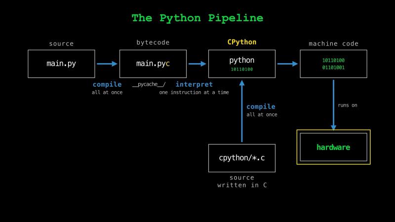
To tell a computer what to do, your code has to be translated into machine instructions in binary format that the hardware can execute, and that translation can happen in different ways.

If all of the code is translated before the program runs, it is called compilation. This is like translating an English text into French all at once, before anyone reads it. If the translation happens statement by statement as the program runs, it is called interpretation, like a real-time translator who listens to each sentence and renders it on the fly.

Python is an interpreted language, meaning it is not compiled directly to machine code (purists will point out that Python is a language specification and can be implemented in different ways, but that is a topic for another time). The boundary is a little subtle, because Python source code is first compiled, all at once, to an intermediate format called bytecode. That is what the .pyc files in your __pycache__ folders are, with the c standing for compiled. This bytecode is then interpreted, one instruction at a time, by CPython, the reference implementation of Python written in C.

C, on the other hand, is a compiled language. So before any of our Python runs, the CPython interpreter itself has already been compiled down to machine code that runs directly on the hardware. There are many more compiled and interpreted languages, but in the end they all run on hardware that executes machine instructions in sequence.

If Else

#

Let’s start with branching in Python, the if else statement. An if else lets us take different actions depending on a condition.

1
2
3
4
5
6
7

x = 0
if x > 0:
    print("x is positive")
elif x < 0:
    print("x is negative")
else:
    print("x is zero")

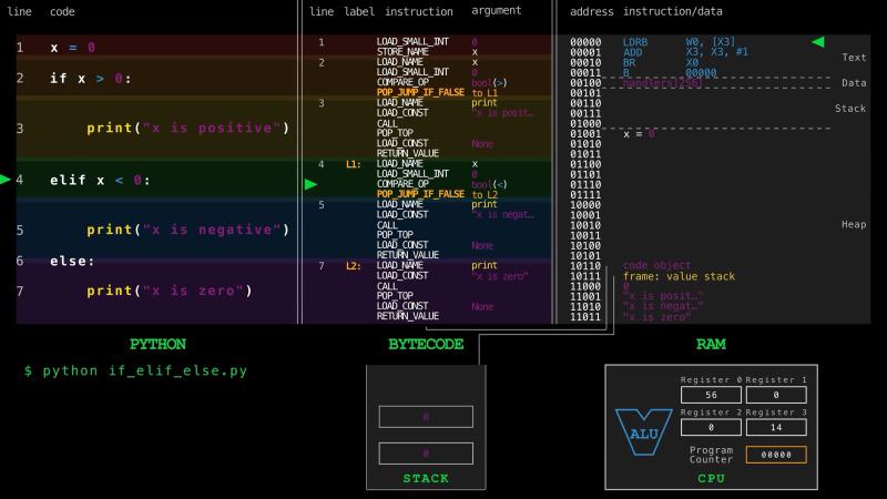
Before we look at the bytecode in detail, let’s briefly explain what a computer does. The Central Processing Unit (CPU) has a little working memory called registers. It has an Arithmetic Logic Unit (ALU) that does the math and comparing. CPU also has an instruction pointer that tracks what to do next. A larger memory (RAM) holds both the instructions and the data they work on. The CPU reads the instruction the pointer is on, runs it, advances the pointer, and repeats. Instructions run one after another.

Python’s disassembler module shows the exact compiled bytecode the CPython interpreter runs. Think of bytecode as the CPython virtual machine’s own instruction set, while the real machine runs binary instructions specific to its hardware.

 1        LOAD_SMALL_INT      0
          STORE_NAME          x
 2        LOAD_NAME           x
          LOAD_SMALL_INT      0
          COMPARE_OP          bool(>)
          POP_JUMP_IF_FALSE   to L1
 3        LOAD_NAME           print
          LOAD_CONST          "x is posit…
          CALL
          POP_TOP
          LOAD_CONST          None
          RETURN_VALUE
 4  L1:   LOAD_NAME           x
          LOAD_SMALL_INT      0
          COMPARE_OP          bool(<)
          POP_JUMP_IF_FALSE   to L2
 5        LOAD_NAME           print
          LOAD_CONST          "x is negat…
          CALL
          POP_TOP
          LOAD_CONST          None
          RETURN_VALUE
 7  L2:   LOAD_NAME           print
          LOAD_CONST          "x is zero"
          CALL
          POP_TOP
          LOAD_CONST          None
          RETURN_VALUE

We trimmed the bytecode of bookkeeping instructions to keep the listings short, and jump targets are written as labels like L1. The number down the left is the source line each group of instructions came from.

Now here is our first puzzle. An if else has to run some instructions and skip others. But we just said the CPU only ever moves to the very next instruction. How can it skip ahead?

The answer is one extra power we already see here, a conditional jump instruction. A conditional jump says, “if this value is false, do not go to the next instruction, go somewhere else instead.” Every branch is a compare followed by POP_JUMP_IF_FALSE, which skips to the next branch when the comparison fails. If you follow the line numbers, you can see the first jump land on the elif or L1, at line 4 and the second land on the else or L2, at line 7. The elif and else are simply the jump targets of the previous check. Machine instructions wield the same conditional jump power, which makes branching possible on any hardware.

Our second puzzle is what else we can do with just conditional and unconditional jump instructions. As it turns out, pretty much all of computation. This is the essence of Turing completeness, and it deserves a chapter of its own. For now, let’s see how the same jump powers while and for loops.

While and For Loops

#

Branching alone is not enough to compute everything. We also need to repeat work, and for that jumps again do the trick.

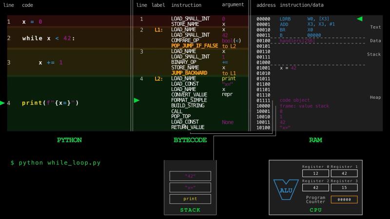
Suppose we have a while loop.

1
2
3
4

x = 0
while x < 42:
    x += 1
print(f"{x=}")

 1        LOAD_SMALL_INT      0
          STORE_NAME          x
 2  L1:   LOAD_NAME           x
          LOAD_SMALL_INT      42
          COMPARE_OP          bool(<)
          POP_JUMP_IF_FALSE   to L2
 3        LOAD_NAME           x
          LOAD_SMALL_INT      1
          BINARY_OP           +=
          STORE_NAME          x
          JUMP_BACKWARD       to L1
 4  L2:   LOAD_NAME           print
          LOAD_CONST          "x="
          LOAD_NAME           x
          CONVERT_VALUE       repr
          FORMAT_SIMPLE
          BUILD_STRING
          CALL
          POP_TOP
          LOAD_CONST          None
          RETURN_VALUE

Let’s reason it out as bytecode instructions. First, store 0 in x. Then check whether x is less than 42. If it is not, jump past the loop body to whatever comes after at L2. If it is, run the body, adding one to x, then jump back up to the check at L1. POP_JUMP_IF_FALSE is our conditional jump out, and JUMP_BACKWARD is our jump back. So, a Python while loop is just a conditional jump to leave, plus an unconditional jump back to do it all again.

A for loop is the same idea in a different form. Instead of checking a condition, it walks an iterator until the iterator runs out.

1
2
3
4

total = 0
for x in range(43):
    total += x
print(total)

 1        LOAD_SMALL_INT      0
          STORE_NAME          total
 2        LOAD_NAME           range
          LOAD_SMALL_INT      43
          CALL
          GET_ITER
    L1:   FOR_ITER            to L2
          STORE_NAME          x
 3        LOAD_NAME           total
          LOAD_NAME           x
          BINARY_OP           +=
          STORE_NAME          total
          JUMP_BACKWARD       to L1
    L2:   ...
 2        POP_ITER
 4        LOAD_NAME           print
          LOAD_NAME           total
          CALL
          POP_TOP
          LOAD_CONST          None
          RETURN_VALUE

FOR_ITER is the conditional jump again. It asks the iterator for the next value, and if there is not one, it jumps out of the loop to L2. Otherwise it binds the value, the body runs, and JUMP_BACKWARD goes back to ask again at L1. Underneath, while and for are the same machine.

Break and Continue

#

The same trick also explains break and continue, the two ways to cut looping short. The break keyword leaves the loop entirely, and continue skips the rest of the current pass and goes straight to the next one.

Take break:

1
2
3
4

for x in range(100):
    if x == 42:
        break
print(x)

 1        LOAD_NAME           range
          LOAD_SMALL_INT      100
          CALL
          GET_ITER
    L1:   FOR_ITER            to L3
          STORE_NAME          x
 2        LOAD_NAME           x
          LOAD_SMALL_INT      42
          COMPARE_OP          bool(==)
          POP_JUMP_IF_TRUE    to L2
          JUMP_BACKWARD       to L1
 3  L2:   POP_TOP
          JUMP_FORWARD        to L4
    L3:   ...
 1        POP_ITER
 4  L4:   LOAD_NAME           print
          LOAD_NAME           x
          CALL
          POP_TOP
          LOAD_CONST          None
          RETURN_VALUE

break is a jump to L4, the instruction after the loop.

continue is its mirror image:

1
2
3
4
5
6

total = 0
for x in range(100):
    if x % 2 == 0:
        continue
    total += x
print(total)

 1        LOAD_SMALL_INT      0
          STORE_NAME          total
 2        LOAD_NAME           range
          LOAD_SMALL_INT      100
          CALL
          GET_ITER
    L1:   FOR_ITER            to L3
          STORE_NAME          x
 3        LOAD_NAME           x
          LOAD_SMALL_INT      2
          BINARY_OP           %
          LOAD_SMALL_INT      0
          COMPARE_OP          bool(==)
          POP_JUMP_IF_FALSE   to L2
 4        JUMP_BACKWARD       to L1
 5  L2:   LOAD_NAME           total
          LOAD_NAME           x
          BINARY_OP           +=
          STORE_NAME          total
          JUMP_BACKWARD       to L1
    L3:   ...
 2        POP_ITER
 6        LOAD_NAME           print
          LOAD_NAME           total
          CALL
          POP_TOP
          LOAD_CONST          None
          RETURN_VALUE

It jumps back to L1 for the next value, skipping the rest of the body. Neither keyword needed new machinery beyond the conditional and unconditional jump instructions we saw.

Try Except

#

Next we look at one of the most important control flow mechanisms in Python: the try except statement. A try except statement in Python lets you attempt something that might fail and handle the failure instead of crashing:

1
2
3
4

try:
    x = int(input("Enter a number: "))
except ValueError:
    print("not a number")

If the user types a number, int parsing succeeds and the except is skipped. If they type something that cannot be converted to an integer, int raises ValueError and control jumps into the handler.

This style is often summarized as “easier to ask forgiveness than permission.” Rather than checking in advance whether every operation will succeed, you try it and handle the failure if it comes. It can read better and save defensive checks.

You may have heard that try except is slow and should be avoided for performance. On modern Python that is a myth. In the bytecode, line 1, the try: itself, compiles to a single NOP, short for no operation, an instruction that does not cost anything to run:

 1        NOP
 2        LOAD_NAME           int
          LOAD_NAME           input
          LOAD_CONST          "Enter a nu…
          CALL
          CALL
          STORE_NAME          x
          LOAD_CONST          None
          RETURN_VALUE
          PUSH_EXC_INFO
 3        LOAD_NAME           ValueError
          CHECK_EXC_MATCH
          POP_JUMP_IF_FALSE   to L1
          POP_TOP
 4        LOAD_NAME           print
          LOAD_CONST          "not a numb…
          CALL
          POP_TOP
          POP_EXCEPT
          LOAD_CONST          None
          RETURN_VALUE
 3  L1:   RERAISE
          COPY
          POP_EXCEPT
          RERAISE

Notice that the happy path runs straight through line 2 and returns. It never even touches the handler instructions below. Instead of branching, the compiler builds a separate exception table off to the side, a map that says “if an instruction in this range raises, here is the handler to jump to.” The cost only arrives when an exception is actually raised and the interpreter looks up where to go. So, try except is usually fine to use for unexpected error handling.

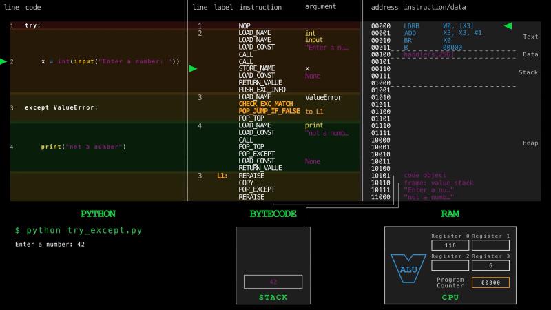
When an exception does fire, picking the right handler is itself a conditional jump. On line 3 of the bytecode listing, CHECK_EXC_MATCH asks whether the raised error matches the ValueError you named, and if it does not, POP_JUMP_IF_FALSE jumps past your handler to L1, where it is re-raised.

try except takes two more clauses. A finally block always runs, whether or not anything failed, which is what you want for cleanup like closing a file. The compiler guarantees this by copying the finally code into both the success and the failure paths. And try can take an else clause, which works just like the else on a loop, so let’s look at both together.

1
2
3
4
5
6
7
8

try:
    x = int(input("Enter a number: "))
except ValueError:
    print("Not a number")
else:
    print(f"You entered {x}")
finally:
    print("Goodbye")

For Else

#

Most of us first meet else attached to an if. But Python also attaches else to loops and to try, and this overloaded meaning can be confusing at first.

A loop’s else runs only if the loop finished normally, without ever hitting a break. Here is the searching for 42 code from before, now with 42 removed from the list, so the loop runs to the end and the else fires:

1
2
3
4
5
6

for n in [4, 8, 15, 16, 23]:
    if n == 42:
        break
else:
    print("42 never showed up")
print("done")

 1        LOAD_CONST          (4, 8, 15, …
          GET_ITER
    L1:   FOR_ITER            to L3
          STORE_NAME          n
 2        LOAD_NAME           n
          LOAD_SMALL_INT      42
          COMPARE_OP          bool(==)
          POP_JUMP_IF_TRUE    to L2
          JUMP_BACKWARD       to L1
 3  L2:   POP_TOP
          JUMP_FORWARD        to L4
    L3:   ...
 1        POP_ITER
 5        LOAD_NAME           print
          LOAD_CONST          "42 never s…
          CALL
          POP_TOP
 6  L4:   LOAD_NAME           print
          LOAD_CONST          "done"
          CALL
          POP_TOP
          LOAD_CONST          None
          RETURN_VALUE

When the loop runs out of items, FOR_ITER jumps to L3, the else block on line 5, and the else runs. But break jumps to L2, which leaps over the else straight to line 6.

This is the classic search-and-report pattern, where you either find a match and break, or fall into the else to report that you never did.

A try else like we saw earlier is similar in spirit to a loop with an else. The else block only runs on normal completion meaning it runs if the try block finishes without raising and without exiting via return, break, or continue.

Bytecode Compiler Optimizations

#

Here is the full example from the intro one more time to mention a few compiler tricks that Python does.

 1
 2
 3
 4
 5
 6
 7
 8
 9
10
11
12

for n in [4, 8, 15, 16, 23, 42]:
    if n == 42:
        print(
            "Answer to the Ultimate Question of Life, "
            f"the Universe, and Everything is {n}."
        )
        break
else:
    print(
        "Yes, Python loops can have an else, "
        "but you won't see this when the loop breaks early"
    )

 1        LOAD_CONST          (4, 8, 15, …
          GET_ITER
    L1:   FOR_ITER            to L3
          STORE_NAME          n
 2        LOAD_NAME           n
          LOAD_SMALL_INT      42
          COMPARE_OP          bool(==)
          POP_JUMP_IF_TRUE    to L2
          JUMP_BACKWARD       to L1
 3  L2:   LOAD_NAME           print
 4        LOAD_CONST          "Answer to …
 5        LOAD_NAME           n
          FORMAT_SIMPLE
          LOAD_CONST          "."
 4        BUILD_STRING
 3        CALL
          POP_TOP
 7        POP_TOP
          LOAD_CONST          None
          RETURN_VALUE
    L3:   ...
 1        POP_ITER
 9        LOAD_NAME           print
10        LOAD_CONST          "Yes, Pytho…
 9        CALL
          POP_TOP
          LOAD_CONST          None
          RETURN_VALUE

Line 1 starts with something odd. We wrote a list, but LOAD_CONST pushes the tuple (4, 8, 15, 16, 23, 42). This is an optimization that avoids the heavier overhead of creating a list at runtime. A mutable list would have to be rebuilt on every run, so the bytecode compiler converted our list into a tuple at compile time and stored it as a constant. We talked about mutable lists and immutable tuples in chapter 2 part 2 of Data Types.

In line 2, we see the LOAD_SMALL_INT instruction, which is a special optimization for small integers. We saw this in Chapter 1, the Object Model. The integers from 0 to 255 are pre-allocated and shared, so the compiler can load them directly without needing to create a new object. In fact, they live in the data section of the process, even though almost all Python objects live in the heap.

For lines 3 to 6, you can see the line column walk into 3, 4, 5, and then back out 4, 3. The f-string is assembled right on the frame’s value stack, with FORMAT_SIMPLE turning the value of n into text and BUILD_STRING joining the pieces at runtime. Notice there are only three pieces. The plain string on line 4 and the opening text of the f-string on line 5 were merged into one constant, because Python joins adjacent string literals at compile time.

So, the compiler does a lot of work to optimize your code before it runs. It folds constants, merges strings, and even inverts the logic of branches to keep the common path fast. But in the end, it is all just instructions that manipulate state and jump around.

Recap

#

In this chapter, we saw that conditional and unconditional jumps make all computation possible. With modifiable state, branching, and iteration, you can compute anything that is computable. Some computations may run too long or need more memory than you have, but those are the only limits.

This also answers the two questions we started with. Any language that gives you branching and iteration can express the same computations, so there is no program you can write in C++ or Rust but not in Python. And any processor with a conditional jump can run them, regardless of architecture. Languages and machines differ in speed, memory, and convenience, not in what they can compute.

But what about functions? We use them all the time, and we just said we do not need them to compute anything. The reverse also turns out to be true. A field called lambda calculus shows that everything we just did with control flow can be done with functions alone.

In the next chapter of our Python Before Production series, we turn to functions. See you there!