PhD in Python Functions

Introduction

#

In this chapter, my goal is to make you an expert in Python functions.

Let’s warm up with a few examples that get progressively trickier.

def add_to_cart(item, cart=[]):
    cart.append(item)
    return cart

alice_cart = add_to_cart("apple")
bob_cart = add_to_cart("banana")

print(alice_cart)
print(bob_cart)

$ python cart.py
['apple', 'banana']
['apple', 'banana']

This mutable default argument gotcha gets repeated so often that most of you probably find it child’s play.

What about this one? We define three functions in a loop, each returning i. What do you think will happen when we call them?

functions = []

for i in range(1, 4):
    def f():
        return i
    functions.append(f)

for f in functions:
    print(f())

Before we look at the output, though, let’s write this compactly using a lambda, which is just a function without a name in Python.

functions = []

for i in range(1, 4):
    functions.append(lambda: i)

for f in functions:
    print(f())

Or even more compactly, using a list comprehension.

for f in [lambda: i for i in range(1, 4)]:
    print(f())

Do you expect the output to be 1, 2, 3?

$ python lambda_loop.py
3
3
3

We get three 3s instead.

Next up, a simple function that prints a global variable.

x = 2026

def show_year():
    print(x)

show_year()

$ python show_year.py
2026

This will output 2026 as expected, no surprises here.

Now, we make a small change: inside the function, right after the print statement, we reassign x to 2027.

x = 2026

def show_year():
    print(x)
    x = 2027

show_year()

Would this still output 2026? Or maybe 2027?

$ python show_year.py
Traceback (most recent call last):
    show_year()
    ~~~~~~~~~^^
    print(x)
          ^
UnboundLocalError: cannot access local variable 'x' where it is not associated with a value

Neither. The print line that worked fine before now raises an error.

By the end of this chapter, instead of memorizing these examples, you will be able to understand and explain why they behave the way they do. But let’s see a couple of harder ones first.

Decorators are a powerful Python feature that lets you change how a function behaves. They’re also a common source of confusion.

Here we have two decorators. What happens when we run this code? Note that we never call f. We’re only defining functions, and f itself does nothing.

def first(_):
    print("1st")

def second(_):
    print("2nd")

@first
@second
def f(): pass

$ python -i decorators.py
2nd
1st
>>>

This output goes against our intuition in two ways. First, we don’t expect function bodies to run without an explicit call. Second, even if we somehow accepted that these two prints happened, the order of execution seems to be reversed.

What if we also called the function f? Would it print anything again?

>>> f()
Traceback (most recent call last):
    f()
    ~^^
TypeError: 'NoneType' object is not callable

We get a runtime error.

We’ll see that decorators aren’t magic. They follow a few simple rules, the same ones that govern how functions work in general.

Things are getting a little spicier now. What happens if we call this function? Will it print Hello and Goodbye? Or just print Hello and stop at the yield?

def my_function():
    print("Hello")
    yield
    print("Goodbye")

my_function()

$ python my_function.py

And it prints… nothing. But don’t worry if you got it wrong, we’ll learn all about generators.

The final boss of this chapter is going to be a function that calculates a running average. We will also learn how Python executes functions under the hood. But we have to work our way up to that level.

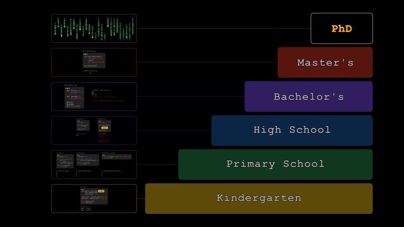
Functions Basics

#

Functions let us wrap up instructions and reuse them with a single call, instead of repeating ourselves (DRY).

They make our code easier to understand, reason about, and test.

For example, given the radius of a circle, we can write functions that calculate its circumference and area.

import math

def get_circumference(radius):
    return 2 * math.pi * radius

def get_area(radius):
    return math.pi * radius ** 2

Functions can receive input and return output, though they don’t need either. But in Python, if a function doesn’t explicitly return a value, it returns None.

def a_function_that_does_nothing(): pass

print(a_function_that_does_nothing())

$ python nothing.py
None

A parameter is the variable listed in the function definition; an argument is the actual value passed in when it’s called. That said, people use the two interchangeably, and you can tell which is which from context.

def train_model(features, target): ...

train_model(X_train, y_train)

You’ll also see *args and **kwargs in function signatures. *args gathers any positional arguments into a tuple, and **kwargs gathers any keyword arguments into a dictionary, so a function can accept any number of arguments.

def show(*args, **kwargs):
    print(args)
    print(kwargs)

show(1, 2, x=3, y=4)

$ python args_kwargs.py
(1, 2)
{'x': 3, 'y': 4}

They show up most often when a function forwards its arguments to another, like a decorator wrapping the function it decorates.

The names are just convention; the * and ** are what matter. When a more descriptive name fits, use it instead of a generic **kwargs:

def load_config(**settings): ...

Functions are first-class citizens in Python, meaning they’re objects, like everything else. We’ll see they can be passed into and returned from other functions. That gives the language a lot of power and flexibility, but the catch is your mental model of functions has to grow. By the end of this chapter, that bigger model will feel natural, because you will understand how functions actually work.

How to Write Functions Well

#

Writing functions well is important, especially so in the age of AI coding. Here are some practical tips.

First off, if you want to blend in with the Python crowd, use_snake_case when naming your functions and variables.

The name should usually start with a verb and tell you what the function does.

def validate_email(): ...
def parse_user(): ...
def train_model(): ...

For example, you can use is, has, or can for functions that return booleans.

def is_valid_email(email): ...
def has_missing_values(df): ...
def can_access_file(user, file): ...

Be consistent with verbs that are common across programming languages.

# Access / retrieval
def get_*: ...       # cheap/local access; retrieve an existing value/entity
def load_*: ...      # read from disk, config, env, or local persisted source
def fetch_*: ...     # retrieve via external I/O, such as DB, API, network, or service call
# Search / database-style retrieval
def find_*: ...      # search for one result; often returns None if not found
def list_*: ...      # retrieve multiple records/items, usually collection-like
def query_*: ...     # build or run a query when query semantics matter
# Construction / conversion / parsing
def create_*: ...    # construct something new from explicit inputs
def from_*: ...      # construct/convert from another representation
def to_*: ...        # convert to another representation or output format
def validate_*: ...  # check correctness; often raises or returns validation result
def parse_*: ...     # convert text/raw input into structured data
def format_*: ...    # convert structured data into string/output form
# Mutation / persistence
def with_*: ...      # return a modified copy without mutating the original
def update_*: ...    # change an existing object/record, often in place or persisted
def save_*: ...      # persist something
def delete_*: ...    # remove something
# Boolean predicates / capability checks
def is_*: ...        # return a boolean property/state
def has_*: ...       # return whether something contains/possesses a thing
def can_*: ...       # return whether an action is allowed/possible

Implementation details can change, so name a function for what it does, not how it does it.

Not great:

def loop_through_logs_and_move_old_ones_to_s3(): ...

Much better:

def archive_old_logs(): ...

Be specific, but strike a balance: avoid names that are too generic or too long.

Not great:

def do_stuff(): ...
def process(data): ...
def handle(): ...
def run(): ...
def calculate_the_accuracy_score_for_the_predictions_given_true_labels(): ...

Much better:

def process_payment(data): ...
def handle_login_failure(): ...
def run_training_pipeline(): ...

Try to avoid abbreviations as they can be confusing.

Not great:

def calc_usr_prf(): ...

Much better:

def calculate_user_performance(): ...

Prefer early returns over nested if/else statements. They keep your logic flat and easy to follow.

Not great:

def can_checkout(user, cart):
    if user.is_active:
        if all(item.is_available for item in cart):
            return True
        else:
            return False
    else:
        return False

Much better:

def can_checkout(user, cart):
    if not user.is_active:
        return False
    if any(not item.is_available for item in cart):
        return False
    return True

Functions should do one thing (Single Responsibility Principle of SOLID). It’s not always clear what “one thing” means, but if you can’t break the function down any further, that’s usually a good sign you’ve captured its single purpose.

Not great:

def pipeline(df):
    df = df.dropna().assign(monthly_spend_log=lambda d: np.log1p(d["monthly_spend"]))
    model = LogisticRegression()
    model.fit(df[["age", "monthly_spend_log"]], df["churn"])
    return model

Much better:

def clean_training_data(df):
    return df.dropna()

def add_churn_features(df):
    return df.assign(monthly_spend_log=lambda d: np.log1p(d["monthly_spend"]))

def train_churn_model(df):
    model = LogisticRegression()
    model.fit(df[["age", "monthly_spend_log"]], df["churn"])
    return model

def pipeline(df):
    df = clean_training_data(df)
    df = add_churn_features(df)
    return train_churn_model(df)

Whenever possible, a function should either modify an object in place or return a new one, not both.

Not great:

def enable_dark_mode(settings):
    settings["theme"] = "dark"
    return settings

Much better:

def enable_dark_mode(settings):
    settings["theme"] = "dark"

or

def with_dark_mode_enabled(settings):
    return settings | {"theme": "dark"}

Last but certainly not least, use type hints. At a minimum, annotate your parameters and return values. Type hints make the function’s expected inputs and outputs clear, help third-party tools catch bugs earlier, and make code easier to read, refactor, and use correctly. We already covered typing in depth in the first chapter of our pip install series.

def with_dark_mode_enabled(settings: dict[str, str]) -> dict[str, str]:
    return settings | {"theme": "dark"}

Function Creation and Scope

#

When you define a function, Python creates a function object in memory.

import math

def get_circumference(radius: int | float) -> float:
    return 2 * math.pi * radius

print(get_circumference(5))

Python passes arguments by assignment. When we call get_circumference(5), Python binds the name radius to the integer object 5. Since 5 is a small integer, it’s already cached in memory, so Python reuses that cached object instead of creating a new one.

If you have experience in other languages, this is neither pure pass-by-reference nor pass-by-value. Python shares the object through a new local name binding. So if you pass a mutable argument, changes you make to it are visible outside the function too.

my_list = [1, 2]

def append_value(target_list: list[int], value: int) -> None:
    target_list.append(value)

append_value(my_list, 3)
print(my_list)

$ python append.py
[1, 2, 3]

As you develop a library or application, you’ll often add functionality to existing functions. For example, we might want to round the output.

import math

def get_circumference(radius: int | float, ndigits: int) -> float:
    return round(2 * math.pi * radius, ndigits)

print(get_circumference(5))

The problem is we just broke all the existing code that calls get_circumference.

$ python circle.py
Traceback (most recent call last):
    print(get_circumference(5))
          ~~~~~~~~~~~~~~~~~^^^
TypeError: get_circumference() missing 1 required positional argument: 'ndigits'

A type checker can flag this without even running the code.

$ ty check circle.py
error[missing-argument]: No argument provided for required parameter `ndigits` of function `get_circumference`
 --> circle.py:6:7
  |
6 | print(get_circumference(5))
  |       ^^^^^^^^^^^^^^^^^^^^
  |
Found 1 diagnostic

Since backward, forward, sideways, and all sorts of compatibility matter in programming, the usual fix is to give ndigits a default value.

import math

def get_circumference(radius: int | float, ndigits: int | None = None) -> float:
    circumference = 2 * math.pi * radius
    if ndigits is None:
        return circumference
    return round(circumference, ndigits)

print(get_circumference(5))  # still works as before
print(get_circumference(5, 2))  # NEW FEATURE!

Here ndigits defaults to None. When Python executes the def statement, it evaluates that default right then. This is called early binding. None is a singleton, already in memory from the moment Python starts, so ndigits just binds to that existing object.

With this knowledge, we are ready to graduate from kindergarten.

In this code, the cart default is created once, when the function is defined, at what people call import time.

def add_to_cart(item, cart=[]):
    cart.append(item)
    return cart

alice_cart = add_to_cart("apple")
bob_cart = add_to_cart("banana")

print(alice_cart)
print(bob_cart)

$ python cart.py
['apple', 'banana']
['apple', 'banana']

The usual way to sidestep this, while still giving each call a brand new list by default, is to use None as a sentinel.

def add_to_cart(item: str, cart: list[str] | None = None) -> list[str]:
    if cart is None:
        cart = []
    cart.append(item)
    return cart

alice_cart = add_to_cart("apple")
bob_cart = add_to_cart("banana")

print(alice_cart)
print(bob_cart)

$ python cart.py
['apple']
['banana']

Back to our circle example. We see different kinds of names here. radius and ndigits are parameters, but there’s also math.pi and round, even though those aren’t parameters.

import math

def get_circumference(radius: int | float, ndigits: int | None = None) -> float:
    circumference = 2 * math.pi * radius
    if ndigits is None:
        return circumference
    return round(circumference, ndigits)

print(get_circumference(5, 2))

The parameters and any name assigned inside the function are its local variables. Here, those are radius, ndigits, and circumference.

If Python can’t find a name in the locals, it looks at the global scope next. In Python, “global” really means module global, not a universal global across the entire program. math is a global object. It lives at module level, outside the function, but we access it inside.

Finally, round is a builtin, a function Python gives you automatically. Unlike math, it doesn’t need an import. To resolve a name like round, Python checks locals first, then globals, then builtins.

Since globals and builtins don’t live in the function’s scope, their values can change between defining the function and calling it. Those names are looked up fresh on every call. This is late binding, the opposite of the early binding we saw with default arguments.

So we can call get_circumference, reassign math.pi to 3, then call it again and get a different result, even though we changed math.pi after defining the function. We can even redefine round entirely, which is called shadowing.

$ python -i circle.py
31.42
>>> print(get_circumference(5))
31.41592653589793
>>> math.pi = 3
>>> print(get_circumference(5))
30
>>> def round(*args, **kwargs): return 0
...
>>> print(get_circumference(5, 2))
0

This is also what happened with our earlier loop. By the time we called the functions, i had already become 3, so all three resolved i to 3.

for f in [lambda: i for i in range(1, 4)]:
    print(f())

$ python comprehension_loop.py
3
3
3

We messed with our globals for learning purposes. Let’s revert them, as a side quest.

Right now round exists in both the globals and the builtins. So if we delete it from the globals, Python falls back to the builtin. That was easy.

>>> del round
>>> print(get_circumference(5, 2))
30

Restoring math.pi is harder, because math is a C extension module. Reloading it doesn’t work, but you can pop it from the module cache and import it fresh.

>>> import importlib
>>> importlib.reload(math)
<module 'math' from '.../math.cpython-314-darwin.so'>
>>> print(get_circumference(5))
30
>>> import sys
>>> sys.modules.pop("math", None)
<module 'math' from '.../math.cpython-314-darwin.so'>
>>> math = importlib.import_module("math")
>>> print(get_circumference(5))
31.41592653589793

All of which is to say: messing with globals and builtins like this is usually a bad idea.

Now we are also ready to understand what’s happening here.

x = 2026

def show_year():
    print(x)
    x = 2027

show_year()

The moment Python sees an assignment to a name anywhere in a function, it treats that name as local for the whole function, even on lines before the assignment. So inside show_year, x is local. But at runtime, print(x) errors, because x is now local and hasn’t been assigned yet.

$ python show_year.py
Traceback (most recent call last):
    show_year()
    ~~~~~~~~~^^
    print(x)
          ^
UnboundLocalError: cannot access local variable 'x' where it is not associated with a value

Without the x = 2027 line, Python wouldn’t treat x as local. It would look it up in the global scope and find 2026, exactly like our first version.

Congratulations on graduating high school.

Decorators

#

We mentioned that functions are objects too, like everything else in Python, which makes them first-class citizens. So we can define functions inside other functions, or pass them around as arguments and return them.

This turns out to be useful when you want to add the same behavior to many functions. For example, say you want to log every call to your fetch_weather and send_notification APIs. The naive way is to add a couple of prints.

def get_users(city):
    ...

def fetch_weather(city, units):
    print(f"calling fetch_weather with {city=}, {units=}")
    ...

def send_notification(user_id, message):
    print(f"calling send_notification with {user_id=}, {message=}")
    ...

city, units = "Berlin", "Celsius"
for user_id in get_users(city):
    message = f"Weather is {fetch_weather(city, units)} degrees {units} in {city}."
    send_notification(user_id=user_id, message=message)

$ python weather.py
calling fetch_weather with city='Berlin', units='Celsius'
calling send_notification with user_id=123, message='Weather is 30 degrees Celsius in Berlin.'
calling fetch_weather with city='Berlin', units='Celsius'
calling send_notification with user_id=456, message='Weather is 29 degrees Celsius in Berlin.'

Note that the fetch_weather API returned a different temperature the second time we called it.

Let’s DRY this further with a log_call function that takes an existing function and returns a new one that wraps it.

def log_call(original_function):
    def new_function(**kwargs):
        kwargs_message = ", ".join(
            f"{key}={value!r}" for key, value in kwargs.items()
        )
        print(f"calling {original_function.__name__} with {kwargs_message}")
        return original_function(**kwargs)
    return new_function

def get_users(city):
    ...

def fetch_weather(city, units):
    ...
fetch_weather = log_call(fetch_weather)

def send_notification(user_id, message):
    ...
send_notification = log_call(send_notification)

fetch_weather(city="Berlin", units="Celsius")

Instead of a couple of print lines, we added many more lines. We can justify this for pedagogical purposes, but in real codebases you should be really careful about over-engineering.

Now, on the right-hand side of fetch_weather = log_call(fetch_weather), we call the already-defined log_call with our original fetch_weather as the argument. Its body runs, but all it does is create the inner new_function. The body of new_function doesn’t run yet, so we see no print output. The name fetch_weather is then rebound to the new function log_call returned. The same story happens with send_notification too. The actual call to fetch_weather() only comes at the end.

The log_call function we just wrote is actually a decorator, and Python gives it special syntax, the @ symbol, to save you from writing function = decorator(function) each time.

def log_call(original_function):
    def new_function(**kwargs):
        kwargs_message = ", ".join(
            f"{key}={value!r}" for key, value in kwargs.items()
        )
        print(f"calling {original_function.__name__} with {kwargs_message}")
        return original_function(**kwargs)
    return new_function

def get_users(city):
    ...

@log_call
def fetch_weather(city, units):
    ...

@log_call
def send_notification(user_id, message):
    ...

fetch_weather(city="Berlin", units="Celsius")

The @ syntax hides everything we just walked through. But now that you’ve seen it once, you know @ before a function is just syntactic sugar, nothing more.

What if we also wanted our logger to track some statistics, like how often each argument value shows up, and log that too?

That’s easy with some containers. Here, two good choices are defaultdict and Counter from the collections module. We place them inside log_call but outside new_function, so they persist separately for each decorated function.

import collections

def log_call(original_function):
    counter_dict = collections.defaultdict(collections.Counter)
    def new_function(**kwargs):
        kwargs_message_list = []
        for key, value in kwargs.items():
            counter_dict[key][value] += 1
            ntimes_called = counter_dict[key][value]
            total = counter_dict[key].total()
            kwargs_message_list.append(f"{key}={value!r} ({ntimes_called}/{total})")
        kwargs_message = ", ".join(kwargs_message_list)
        print(f"calling {original_function.__name__} with {kwargs_message}")
        return original_function(**kwargs)
    return new_function

Now, we can track some calling stats, and we only needed to modify our decorator without touching any decorated functions.

$ python -i weather.py
>>> fetch_weather(city="Paris", units="Celsius")
calling fetch_weather with city='Paris' (1/1), units='Celsius' (1/1)
>>> fetch_weather(city="New York City", units="Fahrenheit")
calling fetch_weather with city='New York City' (1/2), units='Fahrenheit' (1/2)
>>> fetch_weather(city="Rome", units="Celsius")
calling fetch_weather with city='Rome' (1/3), units='Celsius' (2/3)
>>> fetch_weather(city="Istanbul", units="Celsius")
calling fetch_weather with city='Istanbul' (1/4), units='Celsius' (3/4)
>>> send_notification(user_id=123, message="Weather is going to be Sunny today")
calling send_notification with user_id=123 (1/1), message='Weather is going to be Sunny today' (1/1)

Earlier we said functions resolve names through locals, globals, and builtins. So what is counter_dict to new_function? It’s not local, since it’s not created inside new_function, and it’s not global or builtin either. It lives in a fourth scope I held off on until now, which is called Enclosing, the scope of an outer function that wraps an inner one. So when Python resolves a name inside a function, it follows the LEGB rule:

Local      - inside the function
Enclosing  - in a surrounding function, if any
Global     - module-level names
Builtins   - built-in Python names

One side note: because our wrapper only accepts keyword arguments, calling fetch_weather("Istanbul", "Celsius") positionally, without the city= and units= keywords, raises an error.

>>> fetch_weather("Istanbul", "Celsius")
Traceback (most recent call last):
    fetch_weather("Istanbul", "Celsius")
    ~~~~~~~~~~~~~^^^^^^^^^^^^^^^^^^^^^^^
TypeError: log_call.<locals>.new_function() takes 0 positional arguments but 2 were given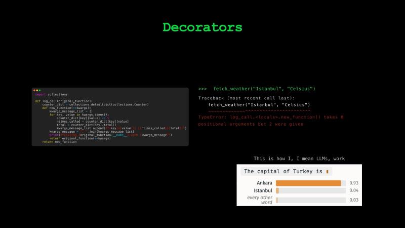

To signal that our API only accepts keyword arguments, we use *, like this:

@log_call
def fetch_weather(*, city, units):
    ...

@log_call
def send_notification(*, user_id, message):
    ...

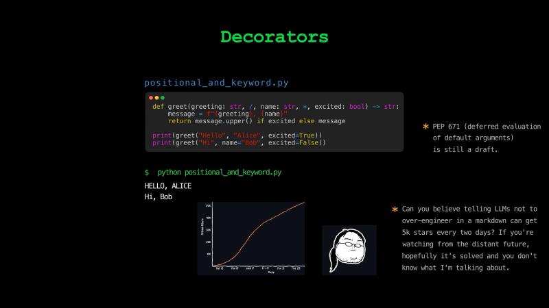
/ does the opposite, forcing the arguments before it to be positional-only. Anything between a / and a * can be passed either way. And this works for any function, plain or decorated.

For example:

def greet(greeting: str, /, name: str, *, excited: bool) -> str:
    message = f"{greeting}, {name}"
    return message.upper() if excited else message

print(greet("Hello", "Alice", excited=True))
print(greet("Hi", name="Bob", excited=False))

$ python positional_and_keyword.py
HELLO, ALICE
Hi, Bob

Here greeting is positional-only, excited must be keyword, and name can go either way.

These / and * markers have more use cases, or they wouldn’t be in the language. Python’s core developers are careful about adding new features.

This is unlike AI agents vibe-coding features nobody asked for.

Because our decorator replaces the original function, we lose some of its metadata, including its docstring, name, and type annotations. To fix that, you can apply functools.wraps, which copies those attributes from the original onto the wrapper.

Without it, help shows the wrapper instead of your original function:

def log_call(original_function):
    def new_function(**kwargs):
        return original_function(**kwargs)
    return new_function

@log_call
def fetch_weather(city, units):
    "Fetch the weather for a city."
    ...

$ python -i wraps_lost.py
>>> help(fetch_weather)
Help on function new_function in module __main__:

new_function(**kwargs)

When you apply @functools.wraps, you get the original name and docstring as expected:

import functools

def log_call(original_function):
    @functools.wraps(original_function)
    def new_function(**kwargs):
        return original_function(**kwargs)
    return new_function

@log_call
def fetch_weather(city, units):
    "Fetch the weather for a city."
    ...

$ python -i wraps_fixed.py
>>> help(fetch_weather)
Help on function fetch_weather in module __main__:

fetch_weather(city, units)
    Fetch the weather for a city.

Decorators can also take arguments. That means another layer in the funception, a function that spits out the decorator based on its arguments.

For example, a file-like argument that says where to log, passed straight through to print():

import sys

def log_call(file):
    def decorator(original_function):
        def new_function(**kwargs):
            print(f"calling {original_function.__name__}", file=file)
            return original_function(**kwargs)
        return new_function
    return decorator

@log_call(file=sys.stderr)
def fetch_weather(*, city, units):
    ...

fetch_weather(city="Berlin", units="Celsius")

Now log_call takes an argument and returns the decorator, so there are three layers instead of two. If you get confused about how this works, you can always lose the syntactic sugar:

fetch_weather = log_call(file=sys.stderr)(fetch_weather)

You’ve been using decorators like these all along, from libraries like FastAPI and Tenacity:

@app.get("/users")
def list_users(): ...

@retry(stop=stop_after_attempt(3))
def fetch_data(): ...

But if your decorator is turning into a monster like this, it’s often cleaner to write it as a class instead of a function. We’ll see how in a future chapter.

Finally, you can stack multiple decorators. Just remember they compose like math functions, applied from the inside out.

With that rule, we can follow what’s going on in this example.

def first(_):
    print("1st")

def second(_):
    print("2nd")

@first
@second
def f(): pass

$ python decorators.py
2nd
1st

First, notice our “decorators” never do anything with the arguments they receive, which is why we name the parameter _, signaling that we don’t use it. Remember, without the @ syntactic sugar, this is equivalent to:

f = first(second(f))

Initially, second(f) runs, so it is actually called. The @ syntax is hiding the function call. After second runs and prints, it implicitly returns None. It never even defines an inner function like a normal decorator would. Then first receives that None and, just like second, ignores it, prints 1st, and returns None. So f isn’t a function anymore, it’s just bound to None. That’s why calling f() raises a TypeError.

Pat yourself on the back, this was your college graduation. Sometimes it’s cooler not to be a college dropout.

Recursion

#

When a big, first-mover company tells you it’s hopeless to compete with them, how would you reason about that decision?

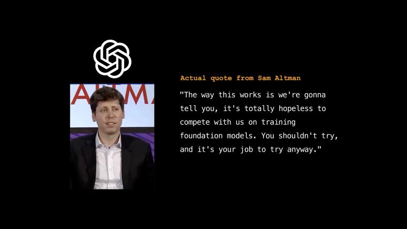
Game theory helps us model strategic interaction. Here, we can use an extensive-form game between two players: an Entrant and an Incumbent. The Entrant moves first and decides whether to enter the market. If it stays out, the Incumbent keeps its monopoly. So, the Entrant gets 0 and the Incumbent gets 4. Every leaf of the tree shows a payoff for both players. Payoffs have no cardinal meaning; we only care which one is larger, that is, their order. If the Entrant enters, the Incumbent decides how to respond: either fight a price war, which makes them both lose money, or accommodate and share the market half and half.

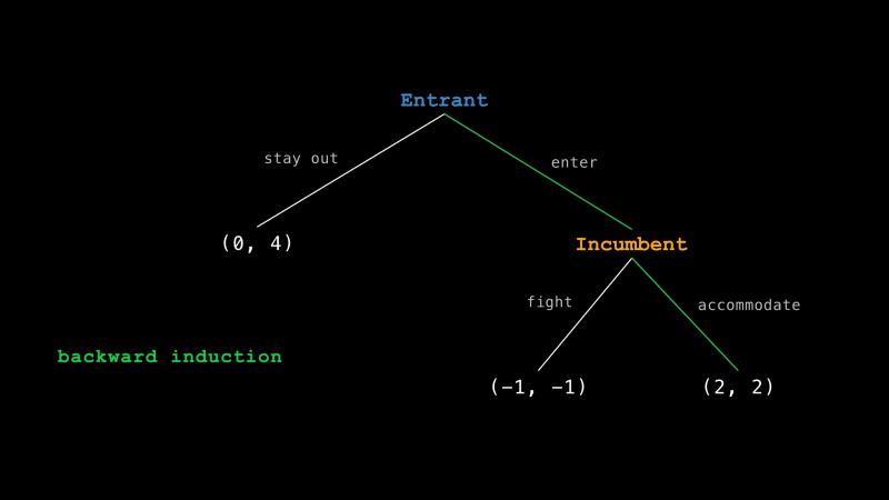
The question then is: standing at the top of this tree, how do we figure out what each player will actually do?

The answer we are looking for is called a Subgame Perfect Nash Equilibrium. It is a set of choices where, in every subtree, or subgame, no player can do better by changing their move, hence the name.

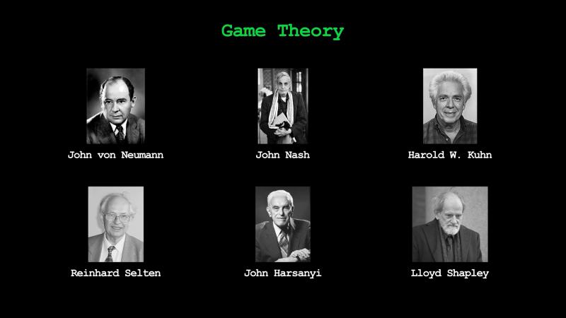
We can find it using a simple algorithm called backward induction. Start at the bottom of the tree, and at each decision let the player take the branch with the best payoff for them, then carry that result up to the node above. In our example, this means that if the Entrant enters, the Incumbent should accommodate, because 2 is larger than -1. Knowing that the Incumbent would accommodate, it is then better for the Entrant to enter than to stay out, since 2 is larger than 0.

But how do we implement backward induction in code? The value of a node depends on the values of the nodes beneath it, which depend on the ones beneath them and so on. A function that solves a node by solving its children is a function that calls itself. This is known as a recursive function.

from collections import namedtuple

Payoff = namedtuple("Payoff", ["entrant", "incumbent"])

game = {
    "player": "entrant",
    "actions": {
        "stay out": Payoff(0, 4),
        "enter": {
            "player": "incumbent",
            "actions": {
                "fight": Payoff(-1, -1),
                "accommodate": Payoff(2, 2),
            },
        },
    },
}

def solve(node):
    if isinstance(node, Payoff):
        return [], node
    player = node["player"]
    best_path, best_payoff = [], None
    for action, branch in node["actions"].items():
        path, payoff = solve(branch)
        if best_payoff is None or getattr(payoff, player) > getattr(best_payoff, player):
            best_path = [(player, action), *path]
            best_payoff = payoff
    return best_path, best_payoff

path, payoff = solve(game)
for player, action in path:
    print(f"{player}: {action}")
print("payoff:", payoff)

$ python game.py
entrant: enter
incumbent: accommodate
payoff: Payoff(entrant=2, incumbent=2)

The solution dives to the bottom of each branch before comparing, then carries the best result back up. This traversal is a depth-first search.

Recursion is powerful, but there’s no free lunch. Take the Fibonacci sequence, where each number is the sum of the two before it.

def fib(n):
    if n < 2:
        return n
    return fib(n - 1) + fib(n - 2)

Our recursive implementation is elegant but extremely slow. We can see why if we count how many nested calls happen inside a single call. How can we do that? Should we print at the start of the function? Or instead, we could just reuse the log_call decorator we wrote earlier.

Back then our decorator only took keyword arguments. fib calls itself positionally, so let’s generalize our decorator to accept *args too, and count each value as it comes in.

import collections

def log_call(original_function):
    counter_dict = collections.defaultdict(collections.Counter)
    args_counter = collections.Counter()
    def new_function(*args, **kwargs):
        message_list = []
        for value in args:
            args_counter[value] += 1
            ntimes_called = args_counter[value]
            total = args_counter.total()
            message_list.append(f"{value!r} ({ntimes_called}/{total})")
        for key, value in kwargs.items():
            counter_dict[key][value] += 1
            ntimes_called = counter_dict[key][value]
            total = counter_dict[key].total()
            message_list.append(f"{key}={value!r} ({ntimes_called}/{total})")
        message = ", ".join(message_list)
        print(f"calling {original_function.__name__} with {message}")
        return original_function(*args, **kwargs)
    return new_function

@log_call
def fib(n):
    if n < 2:
        return n
    return fib(n - 1) + fib(n - 2)

print(fib(30))

$ python fib_naive.py
calling fib with 30 (1/1)
calling fib with 29 (1/2)
calling fib with 28 (1/3)
...
calling fib with 2 (514229/2692535)
calling fib with 1 (832040/2692536)
calling fib with 0 (514229/2692537)
832040

The same values, recomputed over and over, a whopping 2.7 million calls just to get fib(30).

We can fix that with a cache: store each result the first time, then reuse it instead of recomputing the same value. Again, for teaching purposes, we can use a decorator to modify the behavior of a function. Our log_call decorator now lives in its own file, so we import it.

from log_call import log_call

def cache(func):
    results = {}
    def wrapper(n):
        if n not in results:
            results[n] = func(n)
        return results[n]
    return wrapper

@cache
@log_call
def fib(n):
    if n < 2:
        return n
    return fib(n - 1) + fib(n - 2)

print(fib(30))

$ python -i fib_cached.py
calling fib with 30 (1/1)
calling fib with 29 (1/2)
...
calling fib with 0 (1/31)
832040
>>>

Now every value is computed exactly once. We get 31 calls instead of millions. And notice we just stacked two decorators, the same composition we saw earlier. I encourage you to also implement and time both versions. You will see that the function is now tens of thousands of times faster, from one extra decorator.

In your code, you don’t need to write the caching behavior from scratch like we did here. The standard library has functools.cache, which does what we built. There’s also functools.lru_cache, which is the same idea but bounded, keeping only the most recently used results so it can’t grow without limit.

from functools import cache, lru_cache

The cache removes the repeated work, but recursion has another catch. It can go too deep and the stack overflows.

>>> fib(2000)
...
RecursionError: maximum recursion depth exceeded

Python lets you raise that ceiling:

import sys

sys.setrecursionlimit(10000)

Even then, you can still crash the interpreter.

Recursion is elegant, often the most natural way to describe a problem, and genuinely satisfying to write. But in production, the safer move is usually to flatten it, because anything you can express with recursion you can also write as a loop. Here’s a clean non-recursive Fibonacci function. It needs no caching, and no recursion limits to worry about either.

def fib(n):
    a, b = 0, 1
    for _ in range(n):
        a, b = b, a + b
    return a

Generators

#

Python has a built-in range() function, mostly used as a helper for iteration. It’s special because its memory footprint stays tiny, no matter how large the range.

You can give it enormous bounds and it doesn’t load all those numbers into memory. Instead it gives them back one at a time. How can a function pause its execution, and hand control back like that?

Normally a function call is eager in the sense that it runs from start to finish in one go. The yield statement lets a function pause that execution, and if it’s followed by a value, it will hand that value back to the caller before pausing.

from collections.abc import Generator

def my_range(start: int, stop: int, step: int = 1, /) -> Generator[int, None, None]:
    while start < stop:
        yield start
        start += step

This works like range(), except the built-in range makes start optional and accepts more than just ints. One more bit of trivia: range isn’t even a function, it’s an immutable sequence type. But that’s what duck typing is about. range looks and behaves like a function, so everyone calls it one, the official Python docs included.

If you look at the type of my_range we created, it’s a function. Once you call it, you get a generator type.

$ python -i my_range.py
>>> type(my_range)
<class 'function'>
>>> numbers = my_range(1, 4)
>>> type(numbers)
<class 'generator'>

A generator object is an iterator: Python can ask it for values one at a time with the next() function. You’ll sometimes see its type written as Iterator[int] rather than Generator[int, None, None].

>>> next(numbers)
1
>>> next(numbers)
2
>>> next(numbers)
3
>>> next(numbers)
Traceback (most recent call last):
    next(numbers)
    ~~~~^^^^^^^^^
StopIteration

When Python reaches the yield start line, it returns the current value of start to the caller, but it does not destroy the function’s local state. Its local variables, instruction pointer, and execution context are kept alive inside the generator object.

This is why generators are lazy and memory efficient. They do not compute every value ahead of time. They only compute the next value on demand.

The for loop hides this machinery from us:

for number in my_range(1, 4):
    print(number)

It is roughly equivalent to:

numbers = my_range(1, 4)

while True:
    try:
        number = next(numbers)
    except StopIteration:
        break
    print(number)

When it finishes, Python raises StopIteration behind the scenes to signal that there are no more values left, which the for loop handles gracefully.

A lesser-known fact about generators is that they aren’t a one-way street. You can also send a value back into one, where it becomes the result of the yield expression inside. Let’s use that to let the caller rewind our range.

from collections.abc import Generator

def my_range(start: int, stop: int, step: int = 1, /) -> Generator[int, int | None, None]:
    while start < stop:
        step_back = yield start
        if step_back is not None:
            start -= step_back
        start += step

Each Generator has three type parameters: Generator[YieldType, SendType, ReturnType]. Our first version only yielded integers and never received or returned anything, so it was Generator[int, None, None]. This one still yields integers, but now it also receives one through send, or None when you use plain next, so the send type is int | None.

So yield start now does two things at once. It hands start out, and whatever the caller sends back lands in step_back. With next(), nothing is sent, step_back is None, and the range marches forward as before. But send a number and the range steps back by that much first.

$ python -i my_range_send.py
>>> numbers = my_range(1, 4)
>>> next(numbers)
1
>>> next(numbers)
2
>>> numbers.send(1)
2
>>> next(numbers)
3
>>> numbers.send(2)
2
>>> next(numbers)
3

The first call has to be next() or send(None), because there’s no paused yield to receive a value until the generator has started. That first step is called priming the generator.

There’s still the third type parameter we haven’t used. A generator can also return a value when it finishes, separate from what it yields. I’ve never needed this in production, but I’m including it for completeness. Let me know if you’ve ever had a legitimate need for it in your code. We’ll have my_range count how many values it handed out.

from collections.abc import Generator

def my_range(start: int, stop: int, step: int = 1, /) -> Generator[int, int | None, int]:
    count = 0
    while start < stop:
        step_back = yield start
        count += 1
        if step_back is not None:
            start -= step_back
        start += step
    return count

That return value is never yielded, so a for loop or next() won’t give it to you, it’s packed inside the StopIteration that ends the generator. One clean way to read it is yield from, which re-yields every value from another generator and then evaluates to whatever it returned.

from collections.abc import Generator

def logged_range(start: int, stop: int) -> Generator[int, int | None, None]:
    total = yield from my_range(start, stop)
    print(f"yielded {total} values")

print(list(logged_range(1, 4)))

$ python my_range_return.py
yielded 3 values
[1, 2, 3]

And that’s your master’s degree. Because now you can easily reason through why nothing is printed here. We never advanced the generator we got from calling my_function().

def my_function():
    print("Hello")
    yield
    print("Goodbye")

my_function()

$ python my_function.py

But if we did, the first next runs up to the yield and prints Hello. The second resumes, prints Goodbye, falls off the end, and raises StopIteration.

$ python -i my_function.py
>>> gen = my_function()
>>> next(gen)
Hello
>>> next(gen)
Goodbye
Traceback (most recent call last):
    next(gen)
    ~~~~^^^^^
StopIteration

The Theory of Functions

#

This was a long introduction. But you are now ready to see what’s behind the curtain and get your PhD.

So far in this chapter a function has been a practical tool, a way to organize code and build abstractions. But there’s a deeper answer to what a function is, one that goes back to the definition of computation itself.

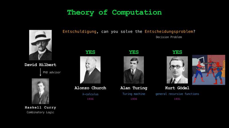
In the 1930s, two people tried to answer the same question: what does it actually mean to compute something? We all have an intuitive sense of algorithms and computation, but can we make it rigorous?

Alan Turing’s answer was his Turing machine, a device with modifiable state on a tape and a list of instructions that read and rewrite it. That’s the same idea at the heart of the von Neumann architecture, the CPU and memory design inside the device you’re using right now. Alonzo Church’s answer seemed completely different. His lambda calculus had no mutable state, just variables, function definition, and application.

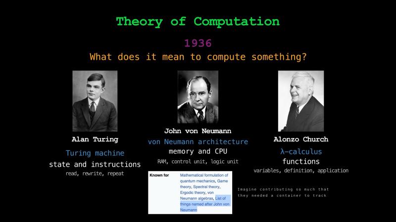
Except the two approaches turned out to be equivalent. Anything you can compute with one model, you can compute with the other, and vice versa. That equivalence backs what’s called the Church-Turing thesis, the claim that these models capture what it means to be computable at all. An interesting fact is that Alonzo Church was Alan Turing’s PhD advisor. Even though they built their theories independently, perhaps they shared some common inspiration.

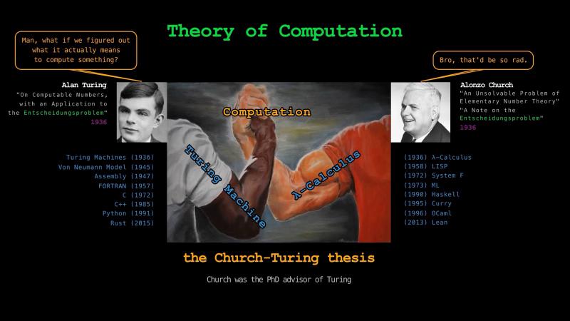
In hardware and most programming languages though, Turing’s theory won. Every mainstream computer is a state-and-instructions machine, not a function-reduction one. Most programming languages are modeled after mutable state and instructions. But Church’s lambda calculus became the center of functional programming.

If you go even deeper, at the root of lambda calculus is combinatory logic, a system that has no bound or quantified variables at all. Someone named Curry worked on combinatory logic extensively. You may have heard of him by his first name.

Haskell Curry’s PhD advisor was “The” David Hilbert. Hilbert posed a million questions that kept all the big brains occupied for more than 100 years and counting, but one of the problems he asked was the decision problem (Entscheidungsproblem), which is what Church and Turing answered independently in 1936. Kurt Gödel had already shown in 1931 that there are true statements in mathematics that cannot be proven, and Church and Turing showed that there are problems that cannot be solved by computation. This was a big blow to Hilbert’s quest to know everything, but that’s for another time.

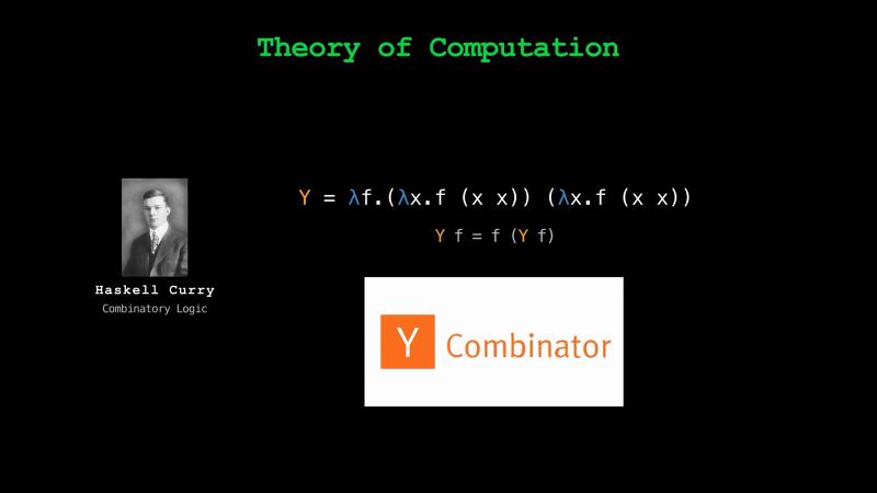
All this history has a lot of loops and rabbit holes of its own. But one of the things Haskell Curry discovered was the Y combinator, which lets pure functions recurse without a name. That’s where the startup accelerator Y Combinator got its name. A company that produces other companies, recursively.

Is Python Object Oriented or Functional?

#

Where does Python sit? Python is, first and foremost, an object-oriented language. I think at this point you’ve heard a dozen times that everything in Python is an object, and also that Python has mutable state and instructions. The CPython interpreter is a virtual CPU executing compiled bytecode. Yet, Python borrows a handful of tools from functional programming.

We’ve already seen two of them: lambdas and closures. There are also partial to freeze some arguments, map, filter, and reduce to transform, select, and collapse a sequence, and singledispatch to run different code depending on a value’s type.

from functools import partial, reduce, singledispatch

def add(x, y):
    return x + y

add_five = partial(add, 5)         # partial: freeze an argument

doubled = list(map(lambda x: x * 2, [1, 2, 3]))           # map: transform
evens = list(filter(lambda x: x % 2 == 0, [1, 2, 3, 4]))  # filter: select
total = reduce(lambda a, b: a + b, [1, 2, 3, 4])          # reduce: collapse

@singledispatch                    # singledispatch: pick code by type
def describe(value):
    return f"something: {value}"

@describe.register
def _(value: int):
    return f"the integer {value}"

None of these make Python a functional language though. They’re useful functional ideas, borrowed into an object-oriented one.

How Python Executes Functions

#

In the last chapter, we learned that Python compiles code to bytecode and the CPython virtual machine runs it one instruction at a time. Functions add the code object and the frame on top of that.

When Python reads a def, it compiles the function body into a code object, which is an immutable bundle of bytecode and constants. The code object of a function is built once and shared by every call. MAKE_FUNCTION wraps that code object into the function you can name and pass around, and CALL is what runs it.

def square(x):
    return x * x

result = square(5)

 1   LOAD_CONST              <code object square>
     MAKE_FUNCTION
     STORE_NAME              square
 4   LOAD_NAME               square
     PUSH_NULL
     LOAD_SMALL_INT          5
     CALL                    1
     STORE_NAME              result

This already explains the first gotcha of the chapter.

def add_to_cart(item, cart=[]):
    cart.append(item)
    return cart

 1   BUILD_LIST              0
     BUILD_TUPLE             1
     LOAD_CONST              <code object add_to_cart>
     MAKE_FUNCTION
     SET_FUNCTION_ATTRIBUTE  defaults
     STORE_NAME              add_to_cart

The BUILD_LIST runs once, at definition time, and the list it makes is attached to the function as its default. Every call that omits cart reuses that one list.

A quick word on the stack data type. A stack is a simple structure. You only add to or grab from the top. This is also known as a LIFO, last in, first out. I’d like to think this is similar to how I handle a hundred open tabs in my browser when I’m researching something. I jump from one topic to another, then return through them one at a time as I finish each. Stacks are widely used in computers. Your CPU keeps a call stack too: calling a function pushes a return address onto it, and returning pops it back off. There’s also stack memory, fast to allocate and organized the same way, as opposed to the heap. Python’s virtual execution model mirrors the hardware.

During function definition you can see decorators being called. Because of the last-in-first-out order of the evaluation stack, the innermost decorator is called first, then the next one, and so on.

@first
@second
def f():
    pass

 1   LOAD_NAME      first
 2   LOAD_NAME      second
 3   LOAD_CONST     <code object f>
     MAKE_FUNCTION
 2   CALL           0          # applies @second, prints "2nd"
 1   CALL           0          # applies @first, prints "1st"
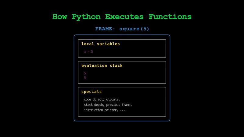
 3   STORE_NAME     f

Each call to a Python function creates a frame of its own. It has three conceptual sections. First, it has local variables. Second, it has its own evaluation stack, where values are pushed and popped as the bytecode runs. And third, it has specials: the bookkeeping the Python interpreter needs to run the frame. This includes the code object, globals dictionary, stack depth, previous frame, instruction pointer, and so on.

Locals in the frame are reached with LOAD_FAST, fast because they’re slots looked up by position, not by name. When show_year only reads x, the compiler loads it as a global:

def show_year():
    print(x)

 2   LOAD_GLOBAL             print
     LOAD_GLOBAL             x

When x = 2027 is in the function body, the load becomes LOAD_FAST_CHECK. This checks if the local slot is filled. At the print line it isn’t yet, which gave us the UnboundLocalError we saw.

def show_year():
    print(x)
    x = 2027

 2   LOAD_GLOBAL             print
     LOAD_FAST_CHECK         x
 3   LOAD_CONST              2027
     STORE_FAST              x

The three-3s closure gotcha happens because the free variable i is read only when the function is called, via LOAD_DEREF.

[lambda: i for i in range(1, 4)]

 1   LOAD_DEREF     i
     RETURN_VALUE

There are two different stacks in play when Python executes your functions. Each frame has its own evaluation stack for operands. The thread has a single call stack, a stack of frames, one per active call. When my_func runs 42 + my_other_func(), it pushes 42 onto its eval stack, then calls my_other_func:

def my_func():
    return 42 + my_other_func()

 2   LOAD_SMALL_INT          42
     LOAD_GLOBAL             my_other_func
     CALL                    0
     BINARY_OP               +

At the CALL, Python pushes a new frame for my_other_func onto the call stack. my_func is now suspended, still holding 42 on its own eval stack. When my_other_func returns, Python pops its frame, follows the link back to my_func, drops the result onto my_func’s eval stack, and the addition finishes. Python keeps these frames in one contiguous per-thread block, tracked by a frame pointer and a stack pointer.

This is also why recursion has a limit. Every call pushes a frame, and a recursive function calls itself, so each level adds another frame to the call stack:

def fib(n):
    if n < 2:
        return n
    return fib(n - 1) + fib(n - 2)

 4   LOAD_GLOBAL             fib
     LOAD_FAST_BORROW        n
     LOAD_SMALL_INT          1
     BINARY_OP               -
     CALL                    1
     LOAD_GLOBAL             fib
     LOAD_FAST_BORROW        n
     LOAD_SMALL_INT          2
     BINARY_OP               -
     CALL                    1
     BINARY_OP               +

A generator’s frame works the same way, but it isn’t allocated in the per-thread call stack; it’s embedded in the generator object itself, which is what lets it outlive a single call. Calling a generator function doesn’t even run the body. The first opcode, RETURN_GENERATOR, hands you the generator object and returns, which is why calling my_function back at the start printed nothing. The body only runs once you advance it, and each yield compiles to YIELD_VALUE. It drops a value back to the caller just like RETURN_VALUE, but instead of discarding the frame it records where it paused, so calling next() or send() again resumes right after the yield.

def gen():
    yield 42

 1   RETURN_GENERATOR        # gen() returns the generator, body not run yet
 2   LOAD_SMALL_INT          42
     YIELD_VALUE

PhD in Python Functions

#

We are now at the final boss: a function that computes a running average. We want it to take an integer and return the average of every integer it has seen so far. This can be implemented in many ways, and we’ll improve our solution step by step, using everything we learned in this chapter.

The obvious first try is to collect the numbers in a list and average them:

from statistics import fmean

values: list[int] = []

def average(value: int) -> float:
    values.append(value)
    return fmean(values)

print(average(10))
print(average(20))
print(average(30))

$ python running_average_naive.py
10.0
15.0
20.0

This works, but values grow forever, consuming more and more memory and slowing the function down as the list gets larger. Since we don’t need the individual numbers, only their average, a running total and a count can give the same answer in constant memory:

total: float = 0.0
count: int = 0

def average(value: int) -> float:
    global total, count
    total += value
    count += 1
    return total / count

print(average(10))
print(average(20))
print(average(30))

$ python running_average_global.py
10.0
15.0
20.0

In order to reassign a global variable from inside a function without UnboundLocalError, we have to declare it as global.

The state is now two globals, and globals are undesirable for many reasons. For example, anything in your program can overwrite total or count, you can only run one average at a time, and globals make the function harder to test. We can instead tuck the state inside a function that returns another function:

from collections.abc import Callable

def make_running_average() -> Callable[[int], float]:
    total = 0.0
    count = 0
    def update_average(value: int) -> float:
        nonlocal total, count
        total += value
        count += 1
        return total / count
    return update_average

average = make_running_average()
print(average(10))
print(average(20))
print(average(30))

Now the state is private to each averager function. The nonlocal keyword is what lets the inner function reassign the enclosing total and count. It’s the closure equivalent of the global keyword. Again, without it, we’re back to UnboundLocalError.

$ python running_average_closure.py
10.0
15.0
20.0

So far, so good. What if we only want the average of the last n numbers, a moving average? We need a sliding window, and the right tool is a deque, pronounced deck. A double-ended queue appends and pops from either end in constant time, and once it’s full it drops the oldest item automatically:

from collections.abc import Callable
from collections import deque
from statistics import fmean

def make_moving_average(n: int) -> Callable[[int], float]:
    window = deque(maxlen=n)
    def update_average(value: int) -> float:
        window.append(value)
        return fmean(window)
    return update_average

average = make_moving_average(2)
print(average(10))
print(average(20))
print(average(30))

$ python moving_average_closure.py
10.0
15.0
25.0

With a window of two, the third value pushes out the first, so the last average is over 20 and 30, which is 25.0.

We could also keep a running total like before and subtract the oldest value when the window is full, but fmean is fast enough for this example and the deque keeps memory usage fixed.

Can we avoid nested functions while keeping the state private? Let’s try it with a generator and send().

from collections import deque
from collections.abc import Generator
from statistics import fmean

def moving_average(n: int) -> Generator[float, int, None]:
    window = deque(maxlen=n)
    while True:
        value = yield fmean(window) if window else 0.0
        if value is not None:
            window.append(value)

average = moving_average(2)
next(average)
print(average.send(10))
print(average.send(20))
print(average.send(30))

$ python moving_average_coroutine.py
10.0
15.0
25.0

You could also hide the next(average) priming behind a decorator, but I’ll leave that as an exercise for you.

An implementation like this shows that you have a solid understanding of Python functions, data types, and control flow. The real wisdom is knowing that this is too much complexity for a simple running average. We have yet to cover Python classes, but they can do the same job with far less ceremony. Or, if you already import third-party data libraries, one of them probably provides an optimized, battle-tested moving average.

And that, is your PhD in Python functions.

Recap

#

In this chapter, we covered a lot about functions.

• Basics of defining and calling functions
• How to write functions well
• Function creation and scope
• Decorators
• Recursion
• Generators
• Theory of computation
• Is Python object-oriented or functional?
• How Python executes functions

Except there’s one kind of function we left out on purpose: async def. This pulls us into different waters: concurrency, parallelism, and the infamous GIL. That’s our next chapter. See you there!